scTour’s cross-data predictions

For version 1.0.0

This tutorial is for version 1.0.0 where prediction functionalities have been separated from inference. Please follow Installation to install the latest version (1.0.0).

Datasets

This notebook shows how to perform cross-data predictions, including predicting the developmental pseudotime, vector field, and latent space of a new dataset. Here one dataset from the developing human cortex is used as training data to train a scTour model. Another three datasets from the developing human cortex, brain organoids, and developing mouse cortex are used as test data.

import sctour as sct
import scanpy as sc
import numpy as np
import pandas as pd
import matplotlib.pyplot as plt

The first dataset (training data, 10X) is from the developing human cortex Trevino et al., 2021, Cell. The same set of cells used in the original study for reconstruction of the excitatory neuron developmental trajectory are used here. This dataset can be downloaded from here.

adata_train = sc.read('../../../../EX_development_data/EX_development_human_cortex_10X.h5ad')
adata_train.shape

(36318, 19073)

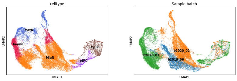
The training dataset has substantial batch effects, as shown below.

sc.pl.umap(adata_train, color=['celltype', 'Sample batch'], legend_loc='on data')

The three test datasets are from the developing human cortex (Drop-seq, Polioudakis et al., 2019, Neuron), brain organoids (10X, Velasco et al., 2019, Nature), and developing mouse cortex (10X, Di Bella et al., 2021, Nature). These three datasets can be downloaded from here.

adata_test1 = sc.read('../../../../EX_development_data/EX_development_human_cortex_DropSeq.h5ad')
adata_test1.shape

(27855, 21655)

adata_test2 = sc.read('../../../../EX_development_data/EX_development_human_organoids_10X.h5ad')
adata_test2.shape

(16032, 17545)

adata_test3 = sc.read('../../../../EX_development_data/EX_development_mouse_cortex_10X.h5ad')
adata_test3.shape

(73649, 16200)

Training

Count the number of genes detected in each cell. This step is required before the scTour model training.

sc.pp.calculate_qc_metrics(adata_train, percent_top=None, log1p=False, inplace=True)

Select the highly variable genes and then use the intersection of these genes with genes detected in all the three test datasets for scTour model training.

sc.pp.highly_variable_genes(adata_train, flavor='seurat_v3', n_top_genes=1000, subset=True, batch_key='Sample batch')
ggs = adata_train.var_names.intersection(adata_test1.var_names).intersection(adata_test2.var_names).intersection(adata_test3.var_names)
adata_train = adata_train[:, ggs]
adata_train.shape

/home/ql312/software/anaconda3/lib/python3.8/site-packages/scanpy/preprocessing/_highly_variable_genes.py:144: FutureWarning: Slicing a positional slice with .loc is not supported, and will raise TypeError in a future version.  Use .loc with labels or .iloc with positions instead.
  df.loc[: int(n_top_genes), 'highly_variable'] = True

(36318, 765)

It’s ready to train the scTour model. Here the model is trained using 60% of all cells.

tnode = sct.train.Trainer(adata_train, percent=0.6)
tnode.train()

Epoch 184: 100%|██████████| 184/184 [27:09<00:00,  8.77s/epoch, train_loss=261, val_loss=260]

Infer the developmental pseudotime, latent space, and vector field based on the trained model.

##pseudotime
adata_train.obs['ptime'] = tnode.get_time()

##latent space
mix_zs, zs, pred_zs = tnode.get_latentsp(alpha_z=0.5, alpha_predz=0.5)
adata_train.obsm['X_TNODE'] = mix_zs

##vector field
adata_train.obsm['X_VF'] = tnode.get_vector_field(adata_train.obs['ptime'].values, adata_train.obsm['X_TNODE'])

Trying to set attribute `.obs` of view, copying.

Generate a new UMAP embedding based on the latent space inferred by scTour.

adata_train = adata_train[np.argsort(adata_train.obs['ptime'].values), :]
sc.pp.neighbors(adata_train, use_rep='X_TNODE', n_neighbors=15)
sc.tl.umap(adata_train, min_dist=0.1)

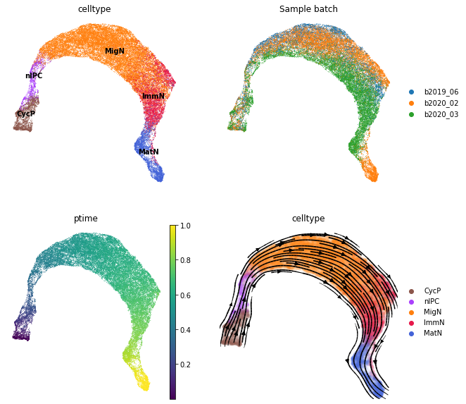
Visualize the inferred pseudotime and vector field on the UMAP. As shown below, all the inferences including the pseudotime, latent representations and vector field from scTour are largely insensitive to batch effects, recapitulating the progression from cycling progenitors to mature excitatory neurons.

fig, axs = plt.subplots(ncols=2, nrows=2, figsize=(10, 10))
sc.pl.umap(adata_train, color='celltype', legend_loc='on data', show=False, ax=axs[0, 0], frameon=False)
sc.pl.umap(adata_train, color='Sample batch', show=False, ax=axs[0, 1], frameon=False)
sc.pl.umap(adata_train, color='ptime', show=False, ax=axs[1, 0], frameon=False)
sct.vf.plot_vector_field(adata_train, zs_key='X_TNODE', vf_key='X_VF', use_rep_neigh='X_TNODE', show=False, ax=axs[1, 1], color='celltype', t_key='ptime', frameon=False, size=80, alpha=0.05)
plt.show()

Save the trained model (optional)

If you prefer to save the trained model for prediction later, please follow the code below to save the model. If you prefer not to save the model, please skip this section and go directly to Prediction section.

##The first parameter is the directory where you want to save the model, and the second parameter is the prefix for the model name.
tnode.save_model(save_dir='./', save_prefix='sctour_model_from_developing_human_brain')

If you have trained a model and saved it, and now you want to use it to predict the cellular dynamics of a query dataset, please follow the code below to load the model before prediction.

tnode = sct.predict.load_model('./sctour_model_from_developing_human_brain.pth')

Prediction

The function sct.predict.predict_time returns the predicted pseudotime based on the model trained.

sct.predict.predict_latentsp function predicts the latent space. Similarly, users can adjust the two parameters alpha_z and alpha_predz based on their purposes. There is a mode parameter in this function, controlling how to predict the latent space by whether or not taking into account the latent space from the training data (default to “fine” to consider the training data). Setting this parameter to “coarse” will ignore the training data.

sct.predict.predict_vector_field function predicts the vector field based on the predicted pseudotime and latent representations.

You might need to adjust the predicted pseudotime and vector field (when you performed post-inference adjustment). Please see section Potential post-inference/prediction adjustment for details.

#test dataset 1
#the first parameter is the trained model
adata_test1.obs['ptime'] = sct.predict.predict_time(tnode, adata_test1)
mix_zs, zs, pred_zs = sct.predict.predict_latentsp(tnode, adata_test1, alpha_z=0.4, alpha_predz=0.6, mode='coarse')
adata_test1.obsm['X_TNODE'] = mix_zs
adata_test1.obsm['X_VF'] = sct.predict.predict_vector_field(tnode, adata_test1.obs['ptime'].values, adata_test1.obsm['X_TNODE'])

#test dataset 2
adata_test2.obs['ptime'] = sct.predict.predict_time(tnode, adata_test2)
mix_zs, zs, pred_zs = sct.predict.predict_latentsp(tnode, adata_test2, alpha_z=0.4, alpha_predz=0.6, mode='coarse')
adata_test2.obsm['X_TNODE'] = mix_zs
adata_test2.obsm['X_VF'] = sct.predict.predict_vector_field(tnode, adata_test2.obs['ptime'].values, adata_test2.obsm['X_TNODE'])

#test dataset 3
adata_test3.obs['ptime'] = sct.predict.predict_time(tnode, adata_test3)
mix_zs, zs, pred_zs = sct.predict.predict_latentsp(tnode, adata_test3, alpha_z=0.4, alpha_predz=0.6, mode='coarse')
adata_test3.obsm['X_TNODE'] = mix_zs
adata_test3.obsm['X_VF'] = sct.predict.predict_vector_field(tnode, adata_test3.obs['ptime'].values, adata_test3.obsm['X_TNODE'])

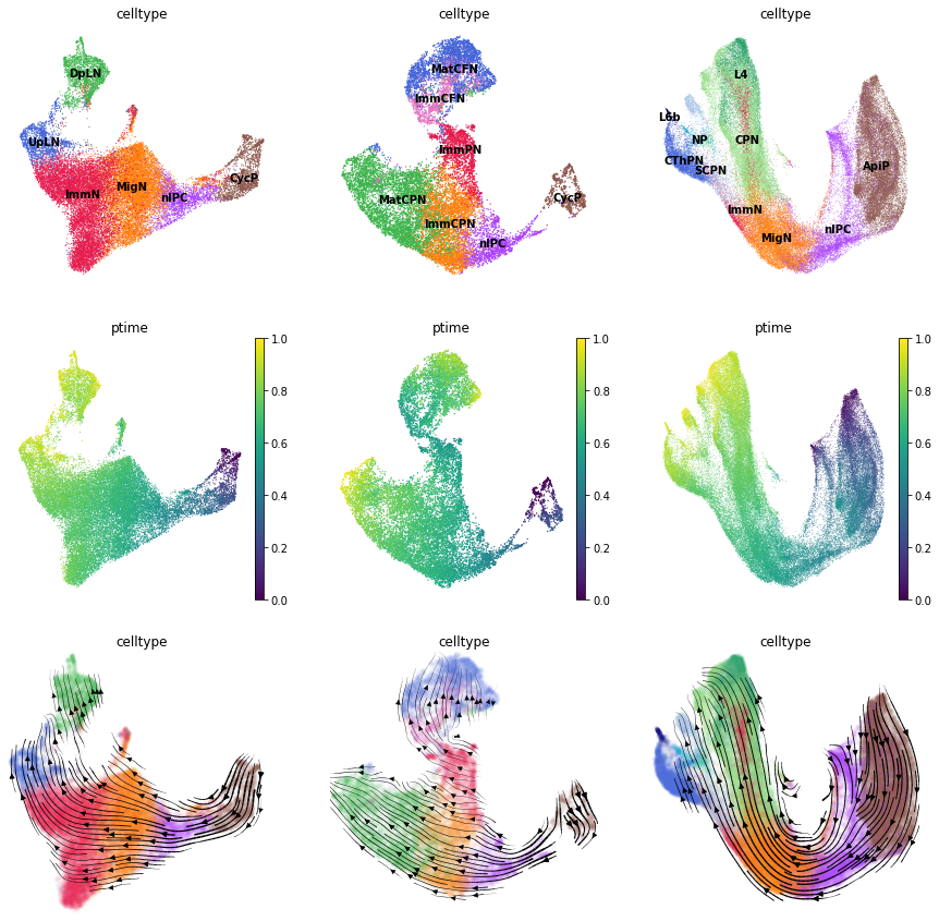
Visualize the predicted pseudotime and vector field for the three test datasets.

fig, axs = plt.subplots(ncols=3, nrows=3, figsize=(15, 15))
for i, adata in enumerate([adata_test1, adata_test2, adata_test3]):
    ##visualize the cell type and predicted pseudotime
    for j, pp in enumerate(['celltype', 'ptime']):
        vmin, vmax = (0, 1) if j == 1 else (None, None)
        sc.pl.umap(adata, color=pp, legend_loc='on data', show=False, ax=axs[j, i], legend_fontsize=10, vmin=vmin, vmax=vmax, frameon=False)
    ##visualize the predicted vector field
    sct.vf.plot_vector_field(adata, zs_key='X_TNODE', vf_key='X_VF', use_rep_neigh='X_TNODE', show=False, ax=axs[2, i], color='celltype', t_key='ptime', legend_loc='none', frameon=False, size=80, alpha=0.05)
plt.show()

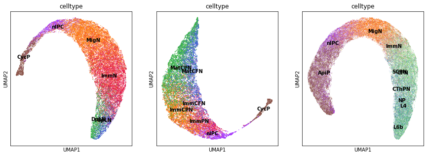
Generate a new UMAP embedding based on the predicted latent space for the three test datasets.

fig, axs = plt.subplots(ncols=3, nrows=1, figsize=(15, 5))
for i, adata in enumerate([adata_test1, adata_test2, adata_test3]):
    adata = adata[np.argsort(adata.obs['ptime'].values), :]
    sc.pp.neighbors(adata, use_rep='X_TNODE', n_neighbors=15)
    sc.tl.umap(adata, min_dist=0.1)
    sc.pl.umap(adata, color='celltype', legend_loc='on data', show=False, ax=axs[i])
plt.show()

Potential post-inference/prediction adjustment

As shown in the scTour inference – Post-inference adjustment tutorial, when the pseudotime/vector field for your training data is returned in reverse order, you need to use the function sct.train.reverse_time to adjust the pseudotime and set the parameter reverse = True in sct.vf.plot_vector_field to adjust the vector field. Correspondingly, you also need to adjust the predicted pseudotime and vector field when this occurs.

For adjusting the predicted pseudotime, you can achieve this in two ways: 1) set the parameter reverse = True in sct.predict.predict_time function; OR 2) use the function sct.train.reverse_time to reverse the returned predicted pseudotime. Either way is able to correct the ordering.

For adjusting the predicted vector field, you need to set the parameter reverse = True when visualizing it using sct.vf.plot_vector_field.